yuca
Step Size is a Consequential Parameter in Continuous Cellular Automata
Experiment with varying step size in an interactive notebook on: mybinder -> ![]() or in colab ->
or in colab -> ![]()
Introduction
Cellular automata (CA) dynamics with continuously-valued states and time steps can be generically written as1:
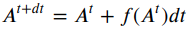
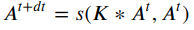
In particular the equation above describes the Lenia framework for continuous CA, and as noted previously in that work 2, the equation above has the same form as Euler’s numerical method for solving differential equations, i.e. estimating CA dynamics if they are described by a differential equation ![]() . CA updates under the Lenia framework are more particularly written as:
. CA updates under the Lenia framework are more particularly written as:
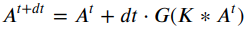
Where ![]() is the grid of cell states at time
is the grid of cell states at time ![]() ,
, ![]() is the growth function,
is the growth function, ![]() is the 2d spatial convolution of neighborhood kernel
is the 2d spatial convolution of neighborhood kernel ![]() with cell states
with cell states ![]() at time
at time ![]() , and
, and ![]() is the step size.
is the step size.
For numerical estimation of differential equations with Euler’s method, error depends on step size. Smaller step sizes typically lead to more accurate solutions. Step sizes that are larger will be less accurate, and if they are too large this can be catastrophic. In the ball drop animation below, simulated with PyBullet 3, the simulation is qualitatively the same across 4 orders of magnitude of step size. It’s not until a time step 100 times larger than PyBullet’s default of 1/240 seconds that catastrophic failure occurs.
Ball drop simulated in pybullet with different time step sizes. Frames are sampled so that animations have the same frame rate, but simulation time step spans 4 orders of magnitude: a) 1/24000 seconds per step, b) 1/2400 seconds per step, c) 1/240 seconds per step (PyBullet default), and d) 1/24 seconds per step.
Ball drop simulated in pybullet with catastrophic (too large) time step size. e) 1/2.4 seconds per step.
Only the final condition with a step size of ~0.4166 seconds displays noticeably non-physical and unstable behavior: the two-wheeled robots plunge through the ground plane before rising slowly like so many spring flowers. Small step sizes behave qualitatively similar to the default, though specific outcomes are noticeably different. In continuous CA, similar differences in step size leads to compromised stability at too small a step size as well as too large. Specific patterns under otherwise identical CA rules occupy different ranges of stable step size. Patterns may also exhibit qualitatively different behaviors at different step sizes. Thus step size choice in continuous CA leads to more interesting differences in outcomes than we see in the PyBullet example and typically expect in numerical physics simulations in general. There are many other physics-based models that support self-organizing solitons, such as chemical reaction-diffusion models (e.g. 4), particle swarms (e.g. 5), or other n-body problems, and these may also exhibit interesting behavioral diversity over a range of step sizes.
Pattern stability depends on step size
A small glider in the style of the
SmoothLife glider 6 and implemented in the Scutium gravidus CA under the Lenia framework is only stable in a range of step sizes from about 0.25 to 0.97. A choice of  outside this range results in a vanishing glider.
A small glider in Lenia’s Scutium gravidus rule set 2, similar to the SmoothLife glider 6, is unstable at step sizes below about 0.25 and above about 0.97.
A wide glider in the same CA rule set is typically stable for over 2000 steps at a ![]() of
of ![]() , but disappears at step sizes of 0.05 or below and is also unstable at a step size of 0.5 or above, usually exhibiting unconstrained growth at large step sizes.
, but disappears at step sizes of 0.05 or below and is also unstable at a step size of 0.5 or above, usually exhibiting unconstrained growth at large step sizes.
A wide glider in Scutium gravidus. Unlike the narrow glider, this glider is pseudo-stable at a moderate step size of 0.1 and unstable for large and small step sizes above and below about 0.5 and 0.05, respectively.
Behavior of individual patterns can vary qualitatively at different step sizes
A more striking consequence of step size is qualitatively different behavior at different step sizes. The following example is a “frog” pattern implemented in an extension of Lenia called Glaberish 7. In Lenia, the growth function ![]() depends only on the results of a 2D convolution of the neighborhood kernel and the cell state grid
depends only on the results of a 2D convolution of the neighborhood kernel and the cell state grid ![]() . Glaberish splits this growth function into persistence (
. Glaberish splits this growth function into persistence (![]() ) and genesis (
) and genesis (![]() ) functions, each contributes to the overal change in cell state according to the current grid states.
) functions, each contributes to the overal change in cell state according to the current grid states.

Glaberish CA dynamics reinstate the dependence on cell state found in SmoothLife, Conway’s Life 8, as well as other Life-like CA, while maintaining the flexibility of Lenia’s growth function. The following frog pattern can be found in a Glaberish CA with evolved persistence ang genesis parameters called s613 (see 9 for details on how this CA was evolved). While the narrow and wide gliders in Lenia’s Scutium gravidus CA occupy particular ranges of ![]() , the s613 frog pattern exhibits qualitatively different behavior across a range of step sizes from about 0.01 to about 0.13.
, the s613 frog pattern exhibits qualitatively different behavior across a range of step sizes from about 0.01 to about 0.13.
For the frog pattern in Glaberish CA s613, varying step size leads to qualitatively different behaviors.
Conclusions
This work demonstrates the consequences of varying step size in continuous CA. Patterns simulated in Lenia’s Scutium gravidus CA are unstable at either too large or too small step size, and different patterns occupy different step size ranges in otherwise identical CA rules. In the Glaberish CA s613, the frog pattern exhibits qualititatively different behavior at step sizes from 0.01 to 0.15, ranging from corkscrewing, meandering, hopping, surging, and finally bursting and disappearing.
The results we have observed for these patterns contrasts sharply with previous remarks concerning the similarity of continuous CA to Euler’s method for solving ODEs with regard to step size 2. Observations of the mobile Orbium pattern in Lenia were consistent with the premise that decreasing step size asymptotically approaches an ideal simulation of the Orbium pattern 2, but for gliders in Scutium gravidus and s613 we have shown that the relationship between CA dynamics and step size is not that simple in general. This work demonstrates that for several patterns a lower step size does not entail a more accurate simulation, but different behavior or potential patterns entirely. Given the evidence presented in this work, it follows that step size should be given due consideration when searching for bioreminiscent patterns 2 10, and for optimization and learning with CA, for example in training patterns to have the agency to negotiate obstacles 11, or for training neural CA for a variety of tasks such as growing patterns 12, classifying pixels 13, learning to generate textures 14, and control 15.
Experiment with varying step size in an interactive notebook on: mybinder -> ![]() or in colab ->
or in colab -> ![]()
This post has not been peer-reviewed itself, but provides supporting information for the following short article accepted to the 2022 Conference on Artificial Life:
- Davis, Q, Tyrell and Bongard, Josh. “Step Size is a Consequential Parameter in Continuous Cellular Automata”. Accepted to The 2022 Conference on Artificial Life. (2022).
References and Footnotes
-
Note: The different formulation for the original, discrete, SmoothLife, which had a discrete time-step (i.e. cell states were replaced at each time step):
 ↩
↩ -
Chan, Bert Wang-Chak. “Lenia - Biology of Artificial Life.” Complex Syst. 28 (2019): https://arxiv.org/abs/1812.05433. ↩ ↩2 ↩3 ↩4 ↩5
-
[https://pybullet.org/][https://pybullet.org/] ↩
-
Munafo, Robert. “Stable localized moving patterns in the 2-D Gray-Scott model.” arXiv: Pattern Formation and Solitons (2014): https://arxiv.org/abs/1501.01990. ↩
-
Schmickl, Thomas et al. “How a life-like system emerges from a simple particle motion law.” Scientific Reports 6 (2016): https://www.nature.com/articles/srep37969 ↩
-
Rafler, Stephan. “Generalization of Conway’s “Game of Life” to a continuous domain - SmoothLife.” arXiv: Cellular Automata and Lattice Gases (2011): https://arxiv.org/abs/1111.1567 ↩ ↩2
-
Davis, Q, Tyrell and Bongard, Josh. “Glaberish: Generalizing the Continuously-Valued Lenia Framework to Arbitrary Life-Like Cellular Automata”. Accepted to The 2022 Conference on Artificial Life. (2022). https://arxiv.org/abs/2205.10463 ↩
-
Gardener, Master. “Mathematical games: the fantastic combinations of john conway’s new solitaire game ‘life’.” (1970). ↩
-
Davis, Q, Tyrell and Bongard, Josh. “Selecting Continuous Life-Like Cellular Automata for Halting Unpredictability: Evolving for Abiogenesis”. Accepted to Proceedings of the Genetic and Evolutionary Computation Conference Companion (2022): https://arxiv.org/abs/2204.07541 ↩
-
Chan, Bert Wang-Chak. “Lenia and Expanded Universe.” ALIFE 2020: The 2020 Conference on Artificial Life. MIT Press, (2020). https://arxiv.org/abs/2005.03742 ↩
-
Hamon, G. and Etcheverry, M. and Chan, B. W.-C. and Moulin-Frier, C. and Oudeyer, P.-Y. Learning sensorimotor agency in cellular automata. Blog post. (2022). https://developmentalsystems.org/sensorimotor-lenia/. ↩
-
Mordvintsev, A. and Randazzo, E. and Niklasson, E. and Levin, M. Growing neural cellular automata. Distill. (2020) https://distill.pub/2020/growing-ca. ↩
-
Randazzo, E. and Mordvintsev, A. and Niklasson, E. and Levin, M. and Greydanus, S. Self-classifying MNIST digits. Distill. (2020) https://distill.pub/2020/selforg/mnist. ↩
-
Niklasson, E. and Mordvintsev, A. and Randazzo, E. and Levin, M. “Self-Organising Textures”, Distill, (2021). https://distill.pub/selforg/2021/textures/ ↩
-
Variengien, A. and Pontes-Filho and Sidny abd Glover, T. and Nichele, S. “Towards self-organized control: Using neural cellular automata to robustly control a cart-pole agent.” Innovations in Machine Intelligence, 1:1–14. (2021). https://arxiv.org/abs/2106.15240v1 ↩