Wrap Your Universe Around a Toroid with Circular Padding Convolutions

Slap Your Universe on a Toroid with Circular Padding

If you’re a cellular automata (CA) enthusiast, you probably already know that you can parameterize arbitrary CA rules as a series of convolutions: one for computing neighborhoods, one for applying CA rules. For a formal example of how this works, check out (Gilpin 2018). But wait! Before you do that, have a look at Distill’s thread on self-organizing systems. As of this writing the thread includes 2 applications of neural cellular automata, and includes interactive examples and code. It’s a good place to get inspired by the current state of CA research.

One thing that I found a bit lacking in my implementations of differentiable (neural) cellular automata is that, with zero-padding, cells behave abnormally at the edges of their universes. Imagine that, while out exploring one day, you reached the edge of our universe and suddenly the laws of physics changed. And not in a cool way either, but in a really lame way that makes everything seem slightly boring. That’s what it’s like to truncate CA universes at the edge of their grid universe, like some sort of common 2D image. Lame! But there is a better way.

Boring!

If you spend any time experimenting with cellular automata software (and you should, try Golly), you’ll notice that many implementations of CA universes wrap around like a game of Pac-Man. Anything exiting stage right re-enters the grid on stage left, and likewise for the top and bottom edges of the grid. There’s a topological way to describe what’s happening: the plane that contains the CA grid actually represents the surface of a toroid. Fun fact: as a deuterostome you too are a toroid. Topologically speaking you are equivalent to a bagel (or a coffee mug).

I was looking at the documentation for torch.nn.Conv2d the other day when I realized we don’t have to embed our CA universes on a boring truncated rectangle. Instead, using padding_mode=circular, we can build unending CA universes by placing them on a toroid. If you’ve already got a PyTorch implementation of cellular automata at home, that’s enough information to make it happen on your own. All you have to do is swap out the current padding mode for "circular". If not, stay tuned for a simple example of implementing John H Conway’s Game of Life on a toroid using PyTorch.

Much better.

If you want to see the code all together in one place, head over to the SortaSota repo to check it out.

After importing PyTorch, Numpy, and matplotlib we’ll be ready to get started.

import numpy as np

import torch
import torch.nn as nn
import torch.nn.functional as F

import matplotlib.pyplot as plt

The first thing we’ll need is to calculate neighborhoods. As we’re implementing Life, we’ll use a Moore neighborhood, which is done by summing up the states of the cells immediately adjacent on all sides (and corners) of a given cell. The neighborhood function is actually where the good stuff happens, making the difference between a toroidal universe and a truncated (boring) flat one. In the code below, setting padding_mode to "circular" is what makes the difference and keeps gliders happily flying foreve (until they crash into chaos and explode, but that’s just Life).

def get_moore_machine(circular=False):

    # conv kernel for calculating a Moore neighborhood
    moore_kernel = torch.tensor([[1,1,1], [1,0,1], [1,1,1]])

    if circular:
        my_mode = "circular"
    else:
        my_mode = "zeros"

    model = nn.Conv2d(1, 1, 3, padding=1, padding_mode=my_mode, bias=False)

    for param in model.named_parameters():
        param[1][0].requres_grad = False

        param[1][0] = moore_kernel

    return model

In Life, live cells with 3 neighbors or less stay alive, and dead cells with exactly 3 neighbors spring into a living state. Everything else transitions to being not-alive. That’s pretty simple to implement in 2 lines of code after we have calculated Moore neighborhoods for our universe. Also notice that since we’re using PyTorch for our CA universe, we can take advantage of all the hardware compatibility and acceleration developed for running deep neural networks. Change device="cpu" to device="cuda" to move your universe from the CPU to run on the GPU with CUDA. I’m moving the new grid back to the CPU in the function below (for plotting), but if you want to take full advantage of GPU speedups you’ll probably want to leave the grid on the GPU or take many steps at once.

def gol_step(my_grid, neighborhood_conv, steps=1, device="cpu"):

    previous_grid = my_grid.float().to(device)

    while steps > 0:

        temp = neighborhood_conv(previous_grid)

        new_grid = torch.zeros_like(previous_grid)

        new_grid[temp == 3] = 1
        new_grid[previous_grid*temp == 2] = 1

        previous_grid = new_grid.clone()

        steps -= 1

    return new_grid.to("cpu")

That’s all the machinery you need to run a toroidal universe according to the rules of Life. If you want to replicate the examples I used to make animations for this post, here is my code invoking and running a Life universe with a few different initializations.

if __name__ == "__main__":

    flat = get_moore_machine()
    toroid = get_moore_machine(circular=True)

    random_grid = torch.randn(64,64) > 0.0

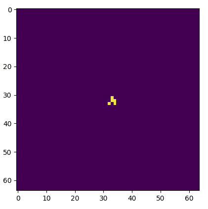
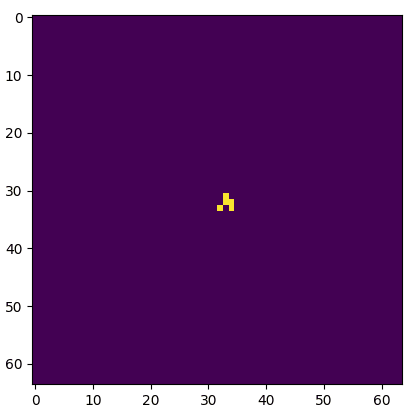
    glider_grid = torch.zeros(64,64)

    glider_grid[32, 32:35] = 1.0
    glider_grid[33, 34] = 1.0
    glider_grid[34, 33] = 1.0

    for my_starting_grid, my_name in zip([random_grid, glider_grid],\
            ["random", "glider"]):

        my_grid = my_starting_grid.clone().unsqueeze(0).unsqueeze(0)


        for step in range(300):

            my_grid = gol_step(my_grid, flat)

            fig = plt.figure()
            plt.imshow(my_grid[0,0,:,:])
            plt.savefig("./flat_gol_{}{}.png".format(my_name, step))
            plt.close(fig)


        my_grid = my_starting_grid.clone().unsqueeze(0).unsqueeze(0)

        for step in range(300):

            my_grid = gol_step(my_grid, toroid)

            fig = plt.figure()
            plt.imshow(my_grid[0,0,:,:])
            plt.savefig("./toroid_gol_{}{}.png".format(my_name, step))
            plt.close(fig)

    print("all done")

And that’s it! Enjoy tinkering with more interesting universes.

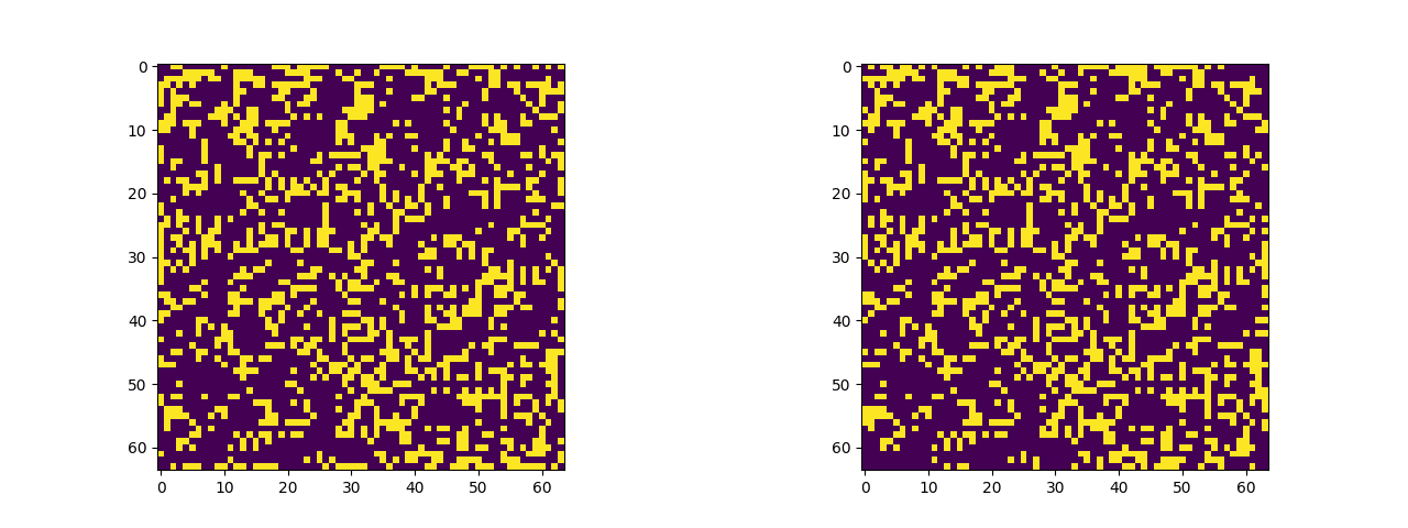
One of these things is not like the other, one of these things just doesn't belong. Actually, in a group of two both are dissimilar. Figuring which is a truncated grid and which uses circular padding is an exercise left to the reader (the starting seed is the same).