The Shapes of Regularization
Introduction
You know you need to regularize your models to avoid overfitting, but what effects does your choice of regularization method have on a model’s parameters? In this tutorial we’ll answer that question with an experiment comparing the effect on parameters in shallow and deep multilayer perceptrons (MLP) trained to classify the digits dataset from scikit-learn under different regularization regimes. The regularization methods we’ll specifically focus on are norm-based parameter penalties, which you may recognize by their Ln nomenclature. Depending on the n, that is, the order of the norm used to regularize a model you may see very different characteristics in the resulting population of parameter values.
If you need a bit of incentive to dive in, consider that regularization is a common topic in interviews, at least insofar as it’s a common line of questioning when I’ve been on the interviewer side of the recruiting table. Of course your life is likely to be much more enjoyable if you are instead driven by the pleasure of figuring things out and building useful tools, but you’ve got to build the base of the pyramid first, of course. Without further ado, let’s get into it.
Let’s start by visualizing and defining norms L0, L1, L2, L3, … L∞
In general, we can describe the Ln norm as
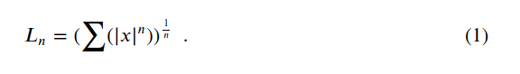
Although we can’t raise the sum in Eq. 1 by the 1/n power when n=0, we can take the limit as n goes to ∞ to find that the L0 norm is 1.0 for all non-zero scalars. In other words, when taking the L0 norm of a vector we’ll get the number of non-zero elements in the vector. The animation below visualizes this process.
As we begin to see for very small values of n, the contribution to the L0 norm for any non-zero value is 1 and 0 otherwise.
If we inspect the figure above we see that there’s no slope to the L0 norm: it’s totally flat everywhere except 0.0, where there is a discontinuity. That’s not very useful for machine learning with gradient descent, but you can use the L0 norm as a regularization term in algorithms that don’t use gradients, such as evolutionary computation, or to compare tensors of parameters to one another. It’s probably not very practical to use with floating point weights in the absence of pruning, but at lower precision or with an active mechanism for zeroing out low-valued weights you may actually incur some zero-valued parameters.
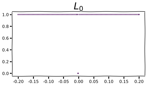
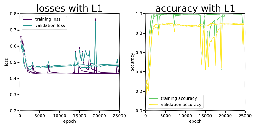
The L1 norm will probably look more familiar and useful.
Visual inspection of the L1 plot reveals a line with a slope of -1.0 before crossing the y-axis and 1.0 afterward. This is actually a very useful observation! The gradient with respect to the L1 norm of any parameter with a non-zero value will be either 1.0 or -1.0, regardless of the magnitude of said parameter. This means that L1 regularization won’t be satisfied until parameter values are 0.0, so any non-zero parameter values better be contributing meaningful functionality to minimizing the overall loss function. In addition to reducing overfitting, L1 regularization encourages sparsity, which can be a desirable characteristic for neural network models for, e.g. model compression purposes.
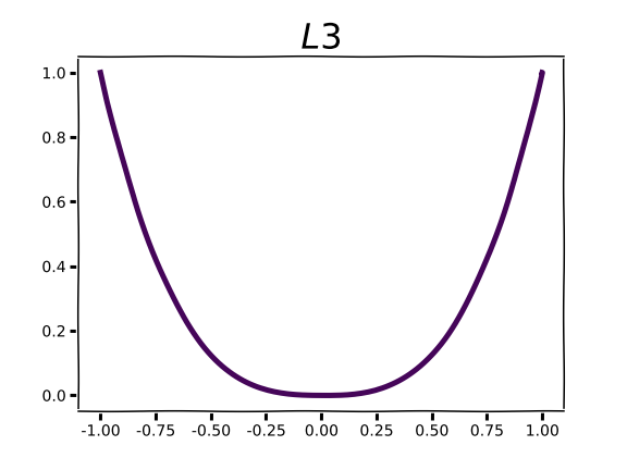
Regularizing with higher order norms is markedly different, and this is readily apparent in the plots for L2 and L3 norms.
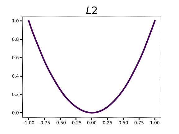
Compared to the sharp “V” of L1, L2 and L3 demonstrate an increasingly flattened curve around 0.0. As you may intuit from the shape of the curve, this corresponds to low gradient values around x=0. Parameter gradients with respect to these regularization functions are straight lines with a slope equal to the order of the norm. Instead of encouraging parameters to take a value of 0.0, norms of higher order will encourage small parameter values. The higher the order, the more emphasis the regularization function puts on penalizing large parameter values. In practice norms with order higher than 2 are very rarely used.
An interesting thing happens as we approach the L∞ norm, typically pronounced as “L sup” which is short for “supremum norm.” The L∞ function returns the maximum absolute parameter value.

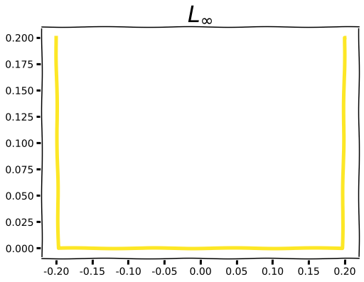
We can visualize how higher order norms begin to converge toward L∞:
Experiment 1
In the previous section we looked at plots for various Ln norms used in machine learning, using our observations to discuss how these regularization methods might affect the parameters of a model during training. Now it’s time to see what actually happens when we use different parameter norms for regularization. To this end we’ll train a small MLP with one hidden layer on the scikit-learn digits dataset. The first experiment will apply Ln from no regularization to n = 3, as well as L∞, to a small fully connected neural network with just one hidden layer. The middle layer is quite wide, so the model ends up with 18,944 weight parameters in total (no biases).
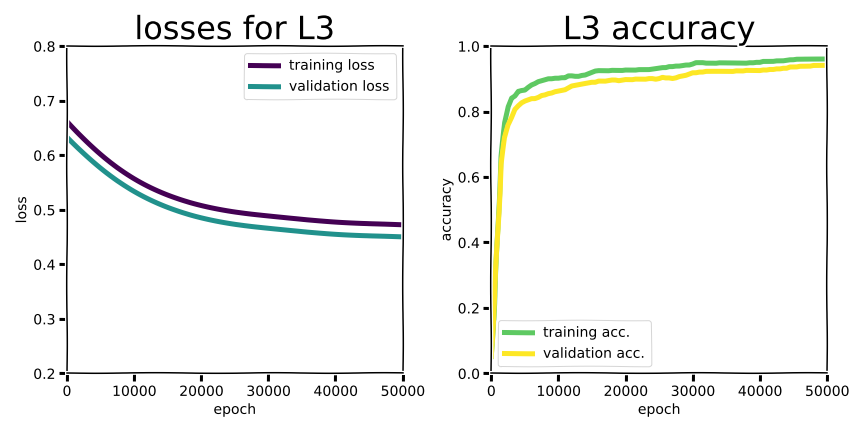
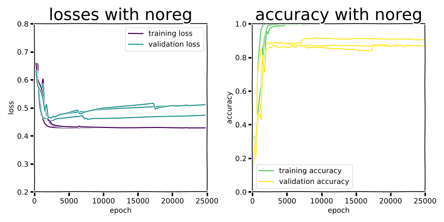
The first thing you might notice in this experiment is that for a shallow network like this, there’s no dramatic “swoosh” pattern in the learning curves for training versus validation data.
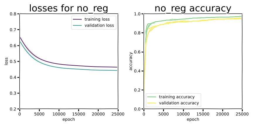
With no regularization there’s only a small gap between training and validation performance at 0.970 +/- 0.001 and 0.950 +/- 0.003 accuracy for training and validation, respectively, for a difference of about 2 percentage points. All margins reported for these experiments will be standard deviation.
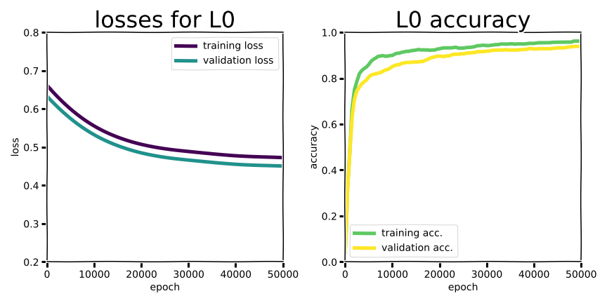
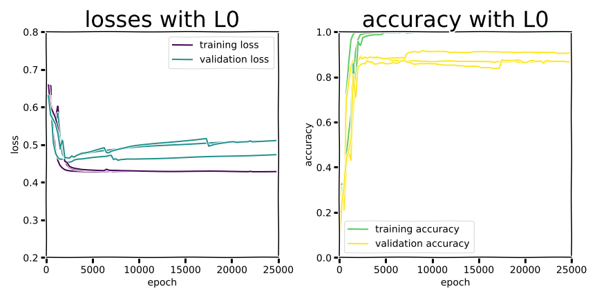
Unsurprisingly L0 regularization is not much different, coming in at 0.97 +/- 0.001 and 0.947 +/- 0.002 and an overfitting gap of about 2.3.
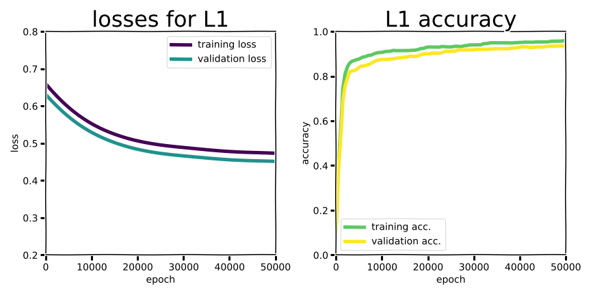
Overfitting for the rest of the Ln regularization strategies remained similarly mild. In fact, for this shallow model overfitting is not that big of a deal, and regularization by penalizing weight values doesn’t make a significant difference.
| Ln | training accurracy | validation accuracy | gap |
|---|---|---|---|
| no reg. | 0.970 +/- 0.001 | 0.950 +/- 0.003 | 0.020 +/- 0.002 |
| L0 | 0.970 +/- 0.001 | 0.947 +/- 0.002 | 0.023 +/- 0.002 |
| L1 | 0.960 +/- 0.001 | 0.938 +/- 0.002 | 0.021 +/- 0.002 |
| L2 | 0.961 +/- 0.002 | 0.934 +/- 0.002 | 0.027 +/- 0.005 |
| L3 | 0.972 +/- 0.002 | 0.951 +/- 0.001 | 0.022 +/- 0.002 |
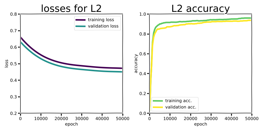
With a shallow network like this regularization doesn’t have a huge impact on performance or overfitting. In fact, the gap between training and validation accuracy was lowest for the case with no regularization at all, barely. What about the effect on the population of model parameters?
| Ln | mean weight mag. | zeros (weights < 1e-3) |
|---|---|---|
| no reg. | 1.24e-2 | 1196 |
| L0 | 1.24e-2 | 1163 |
| L0 | 7.55e-3 | 10412 |
| L0 | 7.58e-3 | 5454 |
| L0 | 1.21e-2 | 1208 |
As we expected from the gradients associated with the various Ln regularization schemes, weights with parameters approximately equal to 0 were most prevalent when using the L1 norm. I was somewhat surprised that L2 also enriched for zeros, but I think this might be an artifact of my choice of cutoff threshold. I’m only reporting statistics for the first seed in each experimental setting, but if you want to run your own statistical analyses in depth I’ve uploaded the experimental results and model parameters to the project repo. You’ll also find the code for replicating the experiments in a jupyter notebook therein.
Experiment 2: Turning it Up to 11 7 Layers
We didn’t see any dramatic overfitting in the first experiment, nor did we graze the coveted 100% accuracy realm. That first model wasn’t really a “deep learning” neural network, sporting a paltry single hidden layer as it did. Might we see more dramatic overfitting with a deep network, perhaps with training accuracies of 1.0 on this small dataset?
In Geoffrey Hinton’s Neural Networks for Machine Learning MOOC originally on Coursera (since retired, but with multiple uploads to YouTube), Hinton supposes researchers tend to agree deep learning begins at about 7 layers, so that’s what we’ll use in this second experiment.
The MLP used in this second experiment has less than half as many parameters as the shallow MLP used earlier at 7,488 weights. The narrow, deep MLP also achieves much higher (training) accuracies for all experimental condition and overfitting becomes a significant issue.
| Ln | training accurracy | validation accuracy | gap |
|---|---|---|---|
| no reg. | 1.00 +/- 0.000 | 0.869 +/- 0.015 | 0.130 +/- 0.015 |
| L0 | 1.00 +/- 0.000 | 0.869 +/- 0.015 | 0.130 +/- 0.015 |
| L1 | 0.997 +/- 0.004 | 0.885 +/- 0.032 | 0.112 +/- 0.033 |
| L2 | 1.00 +/- 0.000 | 0.886 +/- 0.007 | 0.114 +/- 0.007 |
| L3 | 1.00 +/- 0.000 | 0.876 +/- 0.019 | 0.123 +/- 0.019 |
| L∞ | 1.00 +/- 0.000 | 0.882 +/- 0.005 | 0.118 +/- 0.005 |
| dropout | 0.998 +/- 0.001 | 0.893 +/- 0.018 | 0.105 +/- 0.018 |
Experiment 2a, accuracy for `dim_h=32`

Example training curves.
In the second experiment we managed to see dramatic “swoosh” overfitting curves, but validation accuracy was worse across the board than the shallow MLP. There was some improvement in narrowing the training/validation gap for all regularization methods (except L0, which nominally isn’t even differentiable as a discontinuous function), and dropout was marginally better than Ln regularization. Training performance consistently achieved perfect accuracy or close to it, but that doesn’t really matter if a model drops more than 10 percentage points in accuracy at deployment.
Looking at parameter stats might give us a clue as to why validation performance was so bad, and why it didn’t really respond to regularization as much as we would like. In the first experiment, L1 regularization pushed almost 10 times as many weights to a magnitude of approximately zero, while in experiment 2 the difference was much more subtle, with about 25 to 30% more weights falling below the 0.001 threshold than other regularization methods.
| Ln | mean weight mag. | zeros (weights <1e-3) | zeros / noreg zeros |
|---|---|---|---|
| no reg. | 7.01e-2 | 4293 | 1.00 |
| L0 | 7.01e-2 | 4293 | 1.00 |
| L1 | 4.44e-2 | 5420 | 1.26 |
| L2 | 5.92e-2 | 4230 | 0.99 |
| L3 | 6.42e-2 | 4250 | 0.99 |
| L∞ | 5.16e-2 | 4185 | 0.97 |
| dropout | 5.76e-2 | 4377 | 1.02 |
Experiment 2a, weight statistics for deep MLP with `dim_h=32`
This might indicate that the deep model with hidden layer widths of 32 nodes doesn’t have sufficient capacity for redundancy to be strongly regularized. This observation led me to pursue yet another experiment to see if we can exaggerate what we’ve seen so far. Experiment 2b is a variation on experiment 2 with the same deep fully connected network as before but with widely varying width. The skinny variant has hidden layers with 16 nodes, while the wide variant has 256 nodes per hidden layer, just like the shallow network in experiment 1.
| Ln | training accurracy | validation accuracy | gap |
|---|---|---|---|
| no reg. | 1.00 +/- 0.000 | 0.880 +/- 0.019 | 0.120 +/- 0.019 |
| L0 | 1.00 +/- 0.000 | 0.880 +/- 0.019 | 0.120 +/- 0.019 |
| L1 | 1.00 +/- 0.004 | 0.896 +/- 0.005 | 0.104 +/- 0.005 |
| L2 | 1.00 +/- 0.000 | 0.872 +/- 0.005 | 0.128 +/- 0.006 |
| L3 | 1.00 +/- 0.000 | 0.875 +/- 0.021 | 0.124 +/- 0.021 |
| L∞ | 0.999 +/- 0.001 | 0.876 +/- 0.015 | 0.123 +/- 0.016 |
| dropout | 0.401 +/- 0.174 | 0.367 +/- 0.136 | 0.034 +/- 0.051 |
Experiment 2b, accuracy for deep MLP with `dim_h=16`
| Ln | training accurracy | validation accuracy | gap |
|---|---|---|---|
| no reg. | 1.00 +/- 0.000 | 0.933 +/- 0.017 | 0.067 +/- 0.017 |
| L0 | 1.00 +/- 0.000 | 0.933 +/- 0.017 | 0.067 +/- 0.017 |
| L1 | 1.00 +/- 0.004 | 0.937 +/- 0.008 | 0.063 +/- 0.008 |
| L2 | 1.00 +/- 0.000 | 0.949 +/- 0.006 | 0.051 +/- 0.006 |
| L3 | 1.00 +/- 0.000 | 0.940 +/- 0.009 | 0.060 +/- 0.009 |
| L∞ | 1.00 +/- 0.000 | 0.945 +/- 0.009 | 0.055 +/- 0.009 |
| dropout | 1.00 +/- 0.000 | 0.970 +/- 0.002 | 0.030 +/- 0.002 |
Experiment 2b, accuracy for deep MLP with `dim_h=256`
The first thing to notice is that broadening the hidden layers effectively serves as a strong regularization factor over narrow layers, even when no explicit regularization is applied. This may seem counter-intuitive from a statistical learning perspective, as we naturally expect a model with more parameters and thus greater fitting power to overfit more strongly on a small dataset like this. Instead we see that the gap between training and validation accuracy is nearly cut in half when we increased the number of parameters by over 2 orders of magnitude from 2,464 weights in the narrow variant to 346,624 weights in the wide version. Dropout, consistently the most effective regularization technique in experiments 2 and 2b:wide, absolutely craters performance with the deep and narrow variant. Perhaps this indicates that 16 hidden nodes per layer is about as narrow as possible for efficacy on this task.
From my perspective it looks like these results are touching on concepts from the lottery ticket hypothesis (Frankle and Cain 2018), the idea that training deep neural networks isn’t so much a matter of training the big networks per se as it is a search for effective sub-networks. Under the lottery ticket hypothesis it’s these sub-networks that end up doing most of the heavy lifting. The narrow variant MLP just doesn’t have the capacity to contain effective sub-networks, especially when dropout randomly selects only 2/3 of the total search during training.
| Ln | mean weight mag. | zeros (weights <1e-3) | zeros / noreg zeros |
|---|---|---|---|
| no reg. | 1.01e-1 | 1337 | 1.00 |
| L0 | 1.01e-1 | 1337 | 1.00 |
| L1 | 9.64e-2 | 1627 | 1.22 |
| L2 | 8.86e-2 | 1348 | 1.01 |
| L3 | 9.09e-2 | 1341 | 1.00 |
| L∞ | 9.69e-2 | 1337 | 1.00 |
| dropout | 8.81e-2 | 1377 | 1.03 |
Experiment 2b, weight statistics for deep MLP with `dim_h=16`
| Ln | mean weight mag. | zeros (weights <1e-3) | zeros / noreg zeros |
|---|---|---|---|
| no reg. | 6.45e-3 | 228115 | 1.00 |
| L0 | 6.45e-3 | 228115 | 1.00 |
| L1 | 5.97e-3 | 246463 | 1.08 |
| L2 | 6.45e-3 | 227827 | 0.999 |
| L3 | 6.48e-3 | 227991 | 0.999 |
| L∞ | 6.06e-3 | 226845 | 0.994 |
| dropout | 7.63e-3 | 227213 | 0.996 |
Experiment 2b, weight statistics for deep MLP with `dim_h=256`
Although L1 regularization still produces the most weights with a magnitude of approximately zero, it doesn’t match the degree of zero enrichment as experiment 2a, let alone experiment 1. I suspect that this is partially due to my choice of 0.001 as the threshold value for “zero,” and adjusting this lower by a few orders of magnitude would increase the difference in number of zeros for experiment 2 while decreasing the amount of zero enrichment in experiment 1. In any case my first guess that increasing the width of hidden layers would increase the relative enrichment of zeros is proven wrong.
I won’t include plots of training progress for every regularization method in experiment 2b here as they all look pretty much the same (with the exception of the dismal training curve from the narrow variant MLP with dropout). There definitely is an interesting and consistent pattern in learning curves for the wide variant, though, and we’d definitely be remiss not to give it our attention. Look closely and see if you can spot what I’m talking about in the figures below.
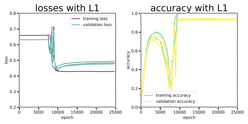
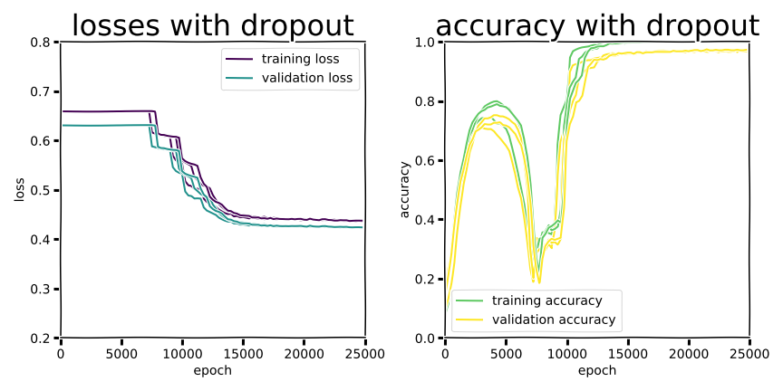
Did you see it? It’s not as smooth as the photogenic plots used in OpenAI’s blog post and paper (Nakkiran et al. 2019), but these training curves definitely display a pattern reminiscent of deep double descent. Note that the headline figures in their work show model size (or width) on the x-axis, but deep double descent can be observed for increasing model size, data, or training time.
Conclusions
What started out as a simple experiment with mild ambitions turned into a more interesting line of inquiry in 3 parts. Our experimental results touched on fundamental deep learning theories like the lottery ticket hypothesis and deep double descent.
I initially intended to simply demonstrate that L1 regularization increases the number of parameters going to zero using a small toy dataset and tiny model. While we did observe that effect our results also speak to making good decisions about depth and width for neural network models. The result that dropout is usually more effective than regularization with parameter value penalties will come as no surprise to anyone who uses dropout regularly, but the emphasis that bigger models can actually yield significantly better validation performance might be counter-intuitive, especially from a statistical learning perspective. Our results did nothing to contradict the wisdom that L1 regularization is probably a good fit when network sparsity is a goal, e.g. when preparing for pruning.
It may be common, meme-able wisdom in deep learning that difficult models can be improved by making them deeper, but as we saw in experiment 2b, deep models are a liability if they are not wide enough. Although we didn’t validate that width is important due to a sub-network search mechanism, our results certainly don’t contradict the lottery ticket hypothesis. Finally, with the wide variant model in experiment 2b we saw a consistent pattern of performance improvement, followed by a loss of performance before finally improving to new heights of accuracy. This might be useful to keep in mind when training a model that apparently sees performance collapse after initially showing good progress. It could be that increasing training time and/or model/dataset size in a situation like that just might push the model over the second threshold on the deep double descent curve.